popeye

What is a population receptive field?

A population receptive field (pRF) is a quantitative model of the cumulative response of the population of cells contained within a single fMRI voxel [1]. The pRF model allows us to interpret and predict the responses of a voxel to different stimuli. Such models can be designed to describe various sensory [2] and cognitive processes [3]. The pRF model has been used to map the retinotopic organization of multiple subcortical nuclei [4].

Installation

Download the popeye source code from the GitHub repository. Links to the tarball and zip files are at the top of this page for your convenience. Using popeye requires that you have installed NumPy, SciPy, statsmodel, Cython, and nibabel. Installing matplotlib is recommended as we'll be plotting the results of our pRF estimation but is not required for any of the model fitting procedures in popeye.

Once you've downloaded the popeye source code and installed the aforementioned dependencies, you'll need to install popeye and build the Cython extensions I've written for speeding up the analyses.

$ cd popeye
$ sudo python setup.py install build_ext
$ cd ~
$ python
>>> import popeye
>>> popeye.__version__
'0.1.0.dev'

Documentation

The code below is meant to provide only a small preview of the purpose and organization of popeye. The full documentation for popeye is available here.

Getting started

Below is a small demonstration of how to interact with the popeye API. Here, we'll generate our stimulus and simulate the BOLD response of a Gaussian pRF model estimate we'll just invent. Normally, we'd be analyzing the BOLD time-series that we collect while we present a participant with a visual stimulus.

import ctypes, multiprocessing
import numpy as np
import sharedmem
import popeye.og_hrf as og
import popeye.utilities as utils
from popeye.visual_stimulus import VisualStimulus, simulate_bar_stimulus

# seed random number generator so we get the same answers ...
np.random.seed(2764932)

### STIMULUS
## create sweeping bar stimulus
sweeps = np.array([-1,0,90,180,270,-1]) # in degrees, -1 is blank
bar = simulate_bar_stimulus(100, 100, 40, 20, sweeps, 30, 30, 10)

## create an instance of the Stimulus class
stimulus = VisualStimulus(bar, 50, 25, 0.50, 1.0, ctypes.c_int16)

### MODEL
## initialize the gaussian model
model = og.GaussianModel(stimulus, utils.double_gamma_hrf)

## generate a random pRF estimate
x = -5.24
y = 2.58
sigma = 1.24
hrf_delay = -0.25
beta = 0.55
baseline = -0.88

## create the time-series for the invented pRF estimate
data = model.generate_prediction(x, y, sigma, hrf_delay, beta, baseline)

## add in some noise
data += np.random.uniform(-data.max()/10,data.max()/10,len(data))

### FIT
## define search grids
# these define min and max of the edge of the initial brute-force search. 
x_grid = (-10,10)
y_grid = (-10,10)
s_grid = (1/stimulus.ppd + 0.25,5.25)
h_grid = (-1.0,1.0)

## define search bounds
# these define the boundaries of the final gradient-descent search.
x_bound = (-12.0,12.0)
y_bound = (-12.0,12.0)
s_bound = (1/stimulus.ppd, 12.0) # smallest sigma is a pixel
b_bound = (1e-8,None)
u_bound = (None,None)
h_bound = (-3.0,3.0)

## package the grids and bounds
grids = (x_grid, y_grid, s_grid, h_grid)
bounds = (x_bound, y_bound, s_bound, h_bound, b_bound, u_bound,)

## fit the response
# auto_fit = True fits the model on assignment
# verbose = 0 is silent
# verbose = 1 is a single print
# verbose = 2 is very verbose
fit = og.GaussianFit(model, data, grids, bounds, Ns=3,
                     voxel_index=(1,2,3), auto_fit=True,verbose=2)

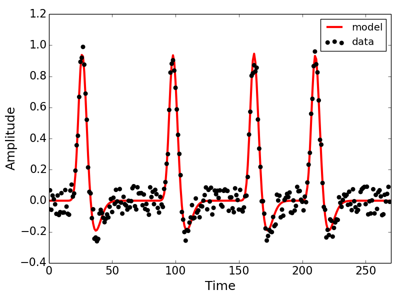
## plot the results
import matplotlib.pyplot as plt
plt.plot(fit.prediction,c='r',lw=3,label='model',zorder=1)
plt.scatter(range(len(fit.data)),fit.data,s=30,c='k',label='data',zorder=2)
plt.xticks(fontsize=16)
plt.yticks(fontsize=16)
plt.xlabel('Time',fontsize=18)
plt.ylabel('Amplitude',fontsize=18)
plt.xlim(0,len(fit.data))
plt.legend(loc=0)

## multiprocess 3 voxels
data = [data,data,data]
indices = ([1,2,3],[4,6,5],[7,8,9])
bundle = utils.multiprocess_bundle(og.GaussianFit, model, data, 
                                   grids, bounds, indices, 
                                   auto_fit=True, verbose=1, Ns=3)

## run
print("popeye will analyze %d voxels across %d cores" %(len(bundle), 3))
with sharedmem.Pool(np=3) as pool:
    t1 = datetime.datetime.now()
    output = pool.map(utils.parallel_fit, bundle)
    t2 = datetime.datetime.now()
    delta = t2-t1
    print("popeye multiprocessing finished in %s.%s seconds" %(delta.seconds,delta.microseconds))

Below is the output of the model fit we invoked in the code block above. Explore the attributes of the fit object to get a sense of the kinds of measures we've gleaned from the model.

Credits

popeye was created by Kevin DeSimone (@kdesimone) with significant contributions and guidance from Ariel Rokem (@arokem).

Support

Having trouble with popeye? Contact kevindesimone@gmail.com

References

[1] Dumoulin SO, Wandell BA (2008) Population receptive field estimates in human visual cortex. NeuroImage 39:647-660.

[2] Thomas JM, Huber E, Stecker E, Boynton G, Saenz M, Fine I (2014) Population receptive field estimates in human auditory cortex. NeuroImage 109: 428:439.

[3] Harvey BM, Klein BP, Petridou N, Dumoulin SO (2013) Topographic organization of numerosity in the human parietal cortex. Science 341: 1123-1126.

[4] DeSimone K, Viviano JD, Schneider KA (2015) Population receptive field estimation reveals two new maps in human subcortex. Journal of Neuroscience 35: 9836-9847.