Getting started
Welcome to popeye! This section of the documentation will help you install popeye and its dependencies and then walks you through a small demonstration of how to use popeye for fitting some simulated timeseries data.
Installation
Download the popeye source code from the GitHub repository here. Using popeye requires that you have installed NumPy, SciPy, statsmodel, Cython, nibabel, and matplotlib. ghpages
Once you’ve downloaded the popeye source code and installed the dependencies, install popeye and build the Cython extensions I’ve written for speeding up the analyses.
$ cd popeye
$ sudo python setup.py install build_ext
$ cd ~ # this ensures we invoke the system install, rather than the cwd
$ python
>>> import popeye
>>> popeye.__version__
'0.1.0.dev'
Demo
Below is a small demonstration of how to interact with the popeye API. Here, we’ll generate our stimulus and simulate the BOLD response of a Gaussian pRF model estimate we’ll just invent. Normally, we’d be analyzing the BOLD time-series that we collect while we present a participant with a visual stimulus.
import ctypes, multiprocessing
import numpy as np
import popeye.og as og
import popeye.utilities as utils
from popeye.visual_stimulus import VisualStimulus, simulate_bar_stimulus

### STIMULUS
## create sweeping bar stimulus
sweeps = np.array([-1,0,-1,90,-1,180,-1,270,-1]) # in degrees, -1 is a blank block
bar = simulate_bar_stimulus(500, 500, 40, 20, sweeps, 30, 30, 10)

## create an instance of the Stimulus class
stimulus = VisualStimulus(bar, 50, 25, 0.25, 1.0, ctypes.c_int16)

### MODEL
## initialize the gaussian model
model = og.GaussianModel(stimulus, utils.double_gamma_hrf)

## generate a random pRF estimate
x = -5.24
y = 2.58
sigma = 1.24
beta = 1
hrf_delay = -0.25

## create the time-series for the invented pRF estimate
data = model.generate_prediction(x, y, sigma, beta, hrf_delay)

## add in some noise
data += np.random.uniform(-data.max()/10,data.max()/10,len(data))

### FIT
## define search grids
# these define min and max of the edge of the initial brute-force search.
x_grid = (-10,10)
y_grid = (-10,10)
s_grid = (0.25,5.25)
b_grid = (0.01,1.0)
h_grid = (-4.0,4.0)

## define search bounds
# these define the boundaries of the final gradient-descent search.
x_bound = (-12.0,12.0)
y_bound = (-12.0,12.0)
s_bound = (0.001,12.0)
b_bound = (1e-8,1e2)
h_bound = (-5.0,5.0)

## package the grids and bounds
grids = (x_grid, y_grid, s_grid, b_grid, h_grid)
bounds = (x_bound, y_bound, s_bound, b_bound, h_bound)

## fit the response
# auto_fit = True fits the model on assignment
# verbose = 0 is silent
# verbose = 1 is a single print
# verbose = 2 is very verbose
fit = og.GaussianFit(model, data, grids, bounds, Ns=3,
                     voxel_index=(1,2,3), auto_fit=True, verbose=2)
Inspecting the results
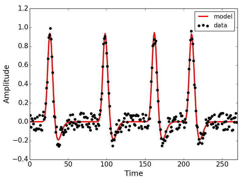
Below is the output of the model fit we invoked in the code block above. We also include some matplotlib code for plotting the simulated data and the predicted timeseries. Explore the attributes of the fit object to get a sense of thekinds of measures gleaned from the pRF model.
## plot the results
import matplotlib.pyplot as plt
plt.plot(fit.prediction,c='r',lw=3,label='model',zorder=1)
plt.scatter(range(len(fit.data)),fit.data,s=30,c='k',label='data',zorder=2)
plt.xticks(fontsize=16)
plt.yticks(fontsize=16)
plt.xlabel('Time',fontsize=18)
plt.ylabel('Amplitude',fontsize=18)
plt.xlim(0,len(fit.data))
plt.legend(loc=0)